Problem with Generic Formulation

As it stands the Generic MDP Formulation in Matlab script is exceedingly slow. Even with some speed ups, it took about 12000 sec ~ 3.3 hours to compile to statistics for the New Graph. I learned from some Matlab forums that vectorization is the key to speedy Matlab scripts. Currently most of my major data structures are matrices, chosen for the ease of debugging readability. However with larger problems come larger data matrices that will be too large to display in Matlab. I might be better off vectorizing everything.

Some Observations About Formulations

1. When the cost of computation is high, the MDP settles down to a deterministic greedy policy. However, there are results that show that the average of the MDP results is slightly worse than the random policy for high computational cost. This suggests that a policy with randomized actions might perform better than a policy with deterministic actions when the optimal metaplanning decision is to make a beeline for the goal. This may also hold for intermediate cases as well. I should look into papers about randomized action policies.

2. I have completed an implementation of the Generic Graph MDP solver. Under this formulation, my states are a 4-tuple consisting of {Arcs Examined, Optimal Quality Level Given Known Information, Current Best Action, Location}. It appears to be working correctly albeit slowly for larger models. I tested it on the original Small Graph and obtain similar results to the Model with 2 Quality Levels in the state tuple. This would suggest that Having multiple quality levels with a minimum arc specification (i.e. current best action) is not necessary. (In a previous blog I comment why it is necessary for multiple quality levels when there is no minimum arc specification).

3. As I see it now, one of the limiting factors for larger graphs is the need to track which arcs have been computed. This is an exponential term 2^(number of arcs) in the complexity, and causes even more problems in the case of generating transition probabilities. No doubt, it will be necessary to do something similar to having QL represent the state of the solution rather than the cost of individual arcs. Perhaps instead of tracking which arcs have been tracked, we can aggregate states by the depth and breadth of the space explored?

Location may also present a problem in the near future. Each location requires the generation of a set of transition probabilities. This can easily get out of hand.

Final QL MDP Results

Here are the final results for the QL MDP. I have also plotted on the same graph the results from the Exact MDP for comparison. As you can see, the QL MDP gives up some performance, and tends to result in a slightly higher total cost than the Exact MDP.

One peculiar behavior that was observed was the that the QL MDP always exhibited compute-move-compute-move-compute-move policies. I wonder if moving helps it eliminate some of the aliasing of the states? Is it intelligently deciding to move to a less ambiguous state?

Problems with State Aliasing

-State aliasing is defined in POMDPs as the phenomenon where several states of the system are aliased to the same observation. It is also referred to as the hidden state problem.

-State aliasing appears in the QL MDP model since several state configurations can map to the same QL. The MDP cannot distinguish between individual underlying states that map to the same QL.

-This creates a problem when it comes time to generate the transition and reward function for the MDP since transitions out of what would normally be distinct states in the Exact model are not blended together.

-One phenomenon that I have observed that confirms this suspicion is the following. I set the costs for all movement actions to be infinite, except when all arcs have been planned. Then I set the cost of movement to be the cost of moving according to the current plan. I also set the cost of planning to be zero. This encourages the MDP to plan all arcs and then to move. Under these circumstances, it makes no difference the order in which that arcs are planned.

-As expected, the policy does perform complete planning before moving. What is peculiar is that the order in which the arcs are planned depends on the graph. Different graph instances result in different arc planning orders. The code is implemented such that it tries computing arcs in order from 1 to 12. It will only swap the order when the value of planning a subsequent arc is strictly greater than the incumbent best arc. So it is expected that since it should make no difference which arc is planned first, the arcs should be planned in order. This behaviour is seen in the Exact MDP model, but not here in the QL model.

-I believe now that the code is implemented correctly. The only reasons I can think of to explain this behavior is that the uniform sampling of the underlying graph worlds is biased in the QL MDP state space toward certain states. So a QL state, which contains multiple underlying states might have some good states blended in with some bad states, reducing the value of the QL state.

Addition of Rewards
-When the rewards are reset to their average values, additional strange behavior occurs. Rather than planning arc 1-12 and then moving, the MDP sometimes decides to plan some, move, plan and move. In most instances this behavior still results in an optimal meta plan. Out of 1000 trial there are about 6-24 instances where this behavior results in reduced plan value.

-Again this is probably due the state aliasing.

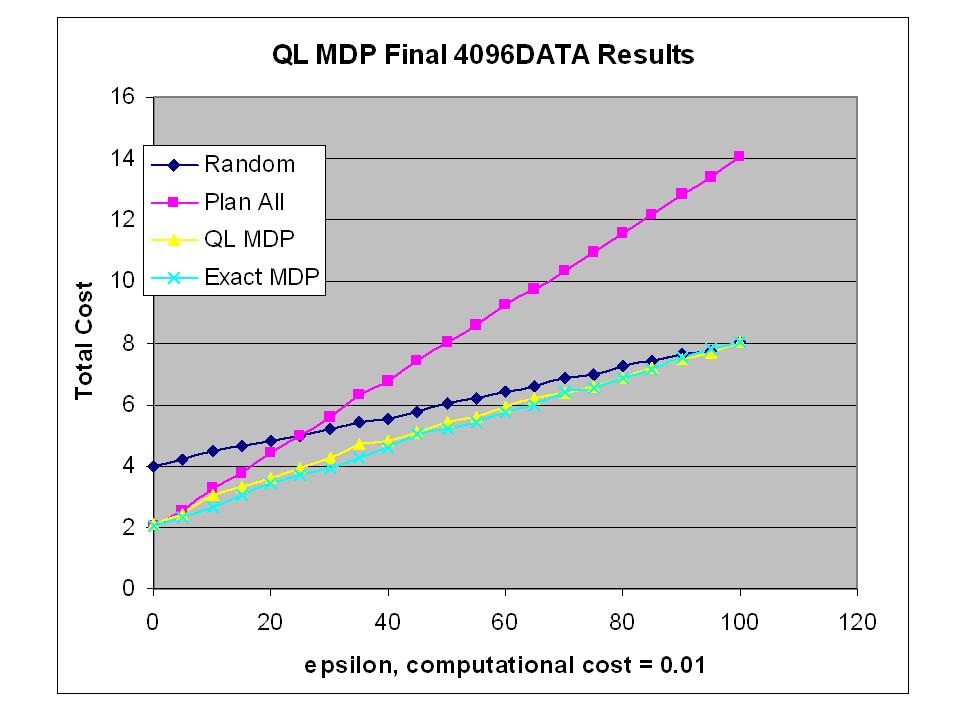
-The next thing that I will do is to generate results for the QL MDP for various epsilons.

Corrected Results for QL on New Graph

These are the first results that look like they make sense for the QL MDP model for the new graph. The one suspicious feature is that the MDP model does not show as dramatic an improvement in this case. Either there is an error or one possibility may be that the number of samples made to determine the transistion probabilities were not enough. I generated 1000 random graphs in order to gather transition probabilities, but there are at least 4096 possible graphs. So I am undersampling. I have various data sets which I will try. These results are for data set 3, where value iteration took 27 sec per iteration, approximately 15 iterations on average. So for 20 different values of computational cost this run took 2.25 hours. Each state is updated during each iteration. I put some logic in there to skip some states with not outgoing transitions to speed up the code. I have another data set that I will try next.
As a sanity check:
It seems to do the right thing when computational costs are high. When computation cost is zero there is s problem. I will investigate.
I also learned that I was handling the sparse matrices incorrectly. In my code I was calculating the transition probability by summing up rows and dividing each column of that row by the sum. The problem was that I was using the find function in Matlab and was repeating the same calculations for each row. The calculations are correct, but I was doing twice the work.
Even so, I think that using sparse matrices will slow down the code, but not to the extent that was happening before

The Case for a Minimum Arc Specification

I am trying to justify the choice of state for my QL formulation. Intially the state only consisted of: {a single quality level to represent the quality of the best solution, the computed arcs, the current location}. This seemed to be obfuscating some states, and I modified my formulation to be {quality level for path along top arc, quality level for path along bottom arc, minimum arc, the computed arcs, the current location}.
I feel that this new formuation does not blend as many underlying states together at the risk of a larger dimentional state space. I have a diagram of the possible choices of combinations of state parameters and plan to discuss them.

Bug in QL MDP for New Graph

Seems as though there is a bug in the QL model. I say this because, it still tends to look at all the arcs with computation cost set to a small positive number. In the Exact MDP implementation it selects a subset of the arcs. I will investigate further.

I also fixed a bug where it was not correctly counting up the arc lengths correctly. I tested it with zero computational cost, and it gets the same answer as the plan all strategy.